Modeling the tyre behaviour – Practical Models
The Magic Formula and the Brush Tyre models
How to model tyre behaviour: brush model tyre.
As we saw in previous chapters, it’s very difficult to describe precisely the behavior of the tyres and that’s the reason why engineers use some models trying to manage the effect of the forces on these “rubber wheels”.
We discuss about the analysis of the properties of a relatively simple theoretical tyre model through a mechanical representation.
This is the case of the Brush Model tyre that is very useful to understand the tyre behavior thanks to its parabolic pressure distribution.
Four fundamental factors play a role in this model: frictional properties in the road-tyre interface, distribution of the normal contact pressure, compliance of the tread rubber and compliance of the belt/carcass.
The fundamentals of brush model tyre.
The simplest model is given by considering a rigid carcass, but there are also more complex ones where the belt is compared to a beam or a string. If the representation of the belt is given by a stretched string instead of an elastic beam, the differential equation model belongs to the second order and not to the fourth.
Brush model tyre parameters.
When the model parameters are chosen properly, the choice of the type of carcass model has only a limited effect. The rigid carcass model with elastic tread elements has a simplicity and qualitative correspondence with experimental tyre behavior. We will consider only a uniform carcass deflection in order to improve the aligning torque representation at combined slip.
The brush model tyre consists of a row of elastic bristles that touches the road plane and can be deflect in a direction parallel to the road surface. Their compliance represents the elasticity of the combination of carcass, belt and actual tread elements of the real tyre.
Brush model formula tyre.
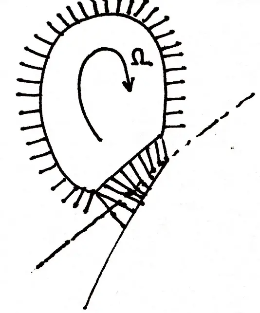
As the tyre rolls, the first element that enters the contact zone is assumed to stand perpendicularly with respect to the road surface. When the tyre rolls freely (no traction or braking forces) and without side slip, camber or turning, the wheel moves along a straight line parallel to the road and in the direction of the wheel plane. In that situation, the tread elements remain vertical and move from the leading edge to the trailing edge without developing a horizontal deflection and consequently without generating a fore and aft or side force.
For further readings and more details see this article pdf.
When the wheel speed vector V shows an angle with respect to the wheel plane, side slip occurs.
\(\begin{align*} \Omega\cdot r_e=V\cdot \cos\alpha \neq V \end{align*} \)Brush model and Magic formula tyre.
Maximum possible deflection that can be reached by the element depending on its position in the contact region. This maximum is governed by the constant coefficient of friction \( \mu \) , the vertical force distribution \( q_z \) and the stiffness of the element \( c_{py} \) . The pressure distribution and consequently also the maximum deflection have been assumed to vary according to a parabola.
As soon as the straight contact line intersects the parabola, sliding will start.
We introduce the slip point S, that is an imaginary point attached to the wheel and is located at the instant considered, a distance equal to the effective rolling radius \( r_e \) below the wheel centre.
At free rolling, by definition, the slip point S has a velocity equal to zero.
Where \( V_r \) is the rolling speed.
Tyre Modeling: the MAGIC Formula tyre model.
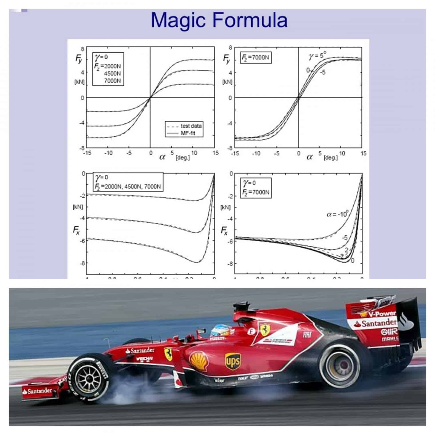
The Magic Formula tyre is a widely used semi-empirical tyre model to calculate steady-state tyre force and moment characteristics for use in vehicle dynamics studies. For the basics about applying the tire-road interaction in Matlab check here.
The general form of the formula for given values of vertical load and camber angle is:
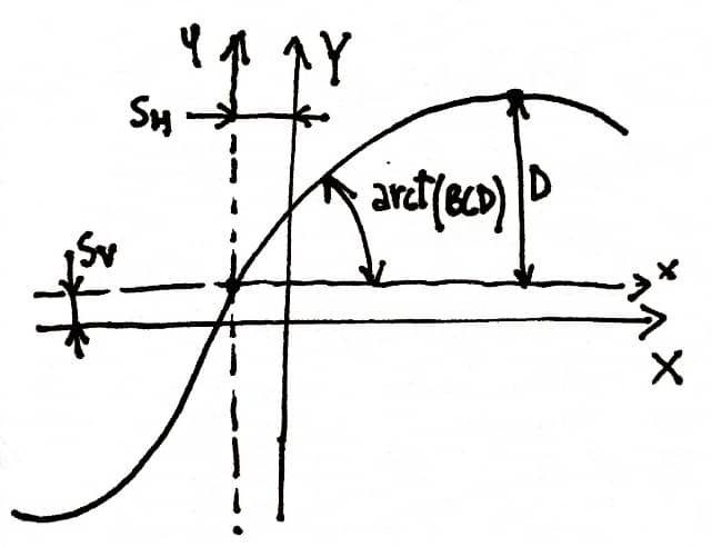
\( \begin{align*} y=D\cdot \sin[C\cdot\arctan(B\cdot x-E\left{B\cdot x- \arctan{B\cdot x}\right{]\end{align*} \)Where:
\( Y(X)= y(x)+S_v \) output variable \( F_x, F_y, F_z \)
\( x= X+S_h \) input variable \( \alpha \) or \( \tan\alpha \)
\( B \) = stiffness factor
\( C \) = shape factor
\( D \) = peak value
\( E \)= curvature factor
\( S_H \) = horizontal shift
\( S_V \) = vertical shift
The Magic Formula \( y(x) \) typically produces a curve that passes through the origin \( x=0, y=0 \) , reaches a maximum and subsequently tends to a horizontal asymptote.


